Categories
FEA

Writing 2D FEA in Python Gh 1

I finally got to write my own FEA code. Always wanted to do so but dreadful because I’m easily distracted and need a good time to focus on this.

Without a background in engineering yet working in an engineering company, I hope writing FEA can help me understand the engineering math.

I mainly follow this article right here and translate it to python. I will eventually upload my code to git but for now I will copy paste the pieces of my code here.

https://podgorskiy.com/spblog/304/writing-a-fem-solver-in-less-the-180-lines-of-code

I use the platform I’m most familiar with, Rhino Grasshopper which have existing methods to define and use mesh. However, I have to use Rhino 5 32bit this time because I want to use numpy for matrix calculation. I have covered the installation in a post below

Inputs

To start a FEA we need boundaries conditions:

A good triangulated mesh

Nodes which are mesh vertices

Support Conditions (nodes that are restrained)

Loading Conditions (loading vectors, loadPts)

Material Info (Poisson Ratio and Young Modulus)

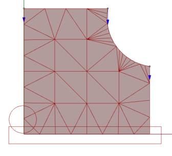
Below is my set up in grasshopper

Set Up

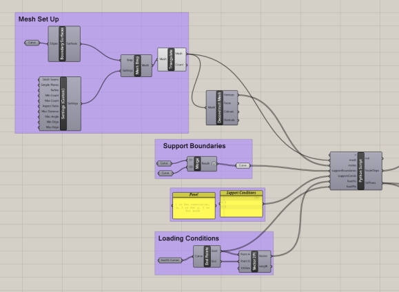
I position the mesh at origin

Set Up 2

Set Up

In order to calculate efficiently, we need to do some “prepping”. We will set up list of nodes, edges, list of loads, list of constraints and list of elements (an element is a triangulated face)

Nodes: The input nodes currently are point3d. However, for convenience, we often refer to the nodes using its index. Whenever the situation arise, I use index to call out the nodes.

Edges: I store the indexes of the line’s start point and end point in a value pair

def GetEdges(mesh):
   edges = [] #list of vertex indices that make up the edges

   for i in range(mesh.TopologyEdges.Count):
       vPair = mesh.TopologyEdges.GetTopologyVertices(i)
       vPairPython = (vPair.I, vPair.J)
       edges.append(vPairPython)
   return edges

Loads: For loads, I need to store them in an array twice the size of the nodes array. Alternate items of the array are X and Y coordinates of the load vector

def GetLoads(nodes, loadPts, loadVs):
     loads = [0] * (len(nodes) * 2)
     for i in range(len(nodes)):
        for j in range(len(loadPts)):
          loadV = loadVs[j]
          dist = rs.Distance(loadPts[j],nodes[i])
          if dist < 0.001:
             loads[2 * i + 0] = loadV.X
             loads[2 * i + 1] = loadV.Y
      return loads

Constraints: I define a class for constraint where type is indicated by integer (1 is for constraint, x, 2 is for y, 3 is for both), node is point3d.

class Constraint:
    def __init__(self, type, node):
        self.Type = type
        self.Node = node
def GetConstraints(supportBoundaries, supportConds, nodes):
    constraints = []

    for i in range(len(nodes)):
        for j in range(len(supportBoundaries)):
           if rs.PointInPlanarClosedCurve(nodes[i], supportBoundaries[j]) == 1:
                con = Constraint(supportConds[j], i)
                constraints.append(con)
    return constraints

Elements: I created Element object woth properties are Nodes and NodeIds

class Element:
      def __init__(self, elemNodes, nodeIds):
           self.Nodes = elemNodes
           self.NodeIds = nodeIds
def GetElements(mesh):
      faceCt = rs.MeshFaceCount(mesh)
      elements = []
      for i in range(faceCt):
         faceVerticeIDs = rs.MeshFaceVertices(mesh)[i]
         nodeIds = faceVerticeIDs[:-1]
         elemNodes = [nodes[nodeIds[0]], nodes[nodeIds[1]], nodes[nodeIds[2]]]
         element = Element(elemNodes, nodeIds)
         elements.append(element)
      return elements

To list out all of them we have:

edges = GetEdges(mesh)
loads = GetLoads(nodes, loadPts, loadVs)
constraints = GetConstraints(supportBoundaries,supportConds, nodes ) #(restraintType, id)
elements = GetElements(mesh)


And…you’re done setting up the items to start on doing some math. I will cover the calculation/matrix manipulations in the next post

Categories
Installation

Install scipy and numpy in Rhino

Hi all,

After a painful process of installling numpy. I would summarize my process as below. Hope it is helpful to everyone.

  1. Download all the egss here. If the link do not work, google “numpy egg enthought”

http://code.enthought.com/.iron/eggs/index.html

Download all of them to your Downloads folder

  1. Follow the instruction here. Follow step 4, 5 ,6 under this link
“C:\Program Files (x86)\IronPython 2.7\ipy.exe” IronPython_numpy_scipy.py --install

It will return an “egginst” error. That’s because you do not have that module yet.

  1. Download ironpkg here

Copy the egginst folder to downloads

  1. Repeat step 2
  2. Modify settings in RhinoPython as step 3 in here
  1. Finally import clr, mtrand, numpy described in the link above. However, please note that this only works in Rhino5 32 bit.
Categories
Computer Vision

yOgA sTrUcT

Although I really enjoy learning, certain topic could be a long and arduous journey which often land me scrolling through the internet looking at dogs and cats or random youtube music videos. Thus, instead of researching or learning a computational topic in depth today, the designer in me decided to write some cheap quick and easy code but able to get something appear on my screen just for the cheap thrill of feeling like a “CoMpUtAtIoNaL DeSiGnEr”.

Beside being a computational designer, I am also a recent practitioner of yoga. While trying out new and more challenging poses, I often find the process of balancing as something iterative. Once finding the balance, the right spot, the pose become much easier and require much less strength. Inspired by the practice, I been trying to bring images of yoga poses photo to a 3D vector skeleton in Rhino.

I run the yoga pose image through two algorithm: poseNet and denseDepth. poseNet returns the human skeleton, with the “coordinates” of the joints. These coordinates are then mapped onto denseDepth image, return us the “brightness” of that pixels. All these numbers are then brought into Rhino and make up a 3D human skeleton.

Gratitude-Asana_Briohny-Smyth_Warrior2

Original Image

PoseNet - December 15th 2019 at 10.20.27 PM

PoseNet

Gratitude-Asana_Briohny-Smyth_Warrior2 Dense Depth

Dense Depth

Gratitude-Asana_DD MappedJts

Dense Depth with mapped joints (zoom in closely)

3D result…sorry for the exploded head hehe.

I understand that there are much better algorithm to do this such as densepose and the result looks very different from the image, but hey this is just an attempt for me to have some fun!

Categories
Mesh

Half-edge mesh

Beside the default mesh that Rhino provide, there’s another type of mesh that is very popular among Rhino, grasshopper developers: Half-edge mesh. The half edge mesh concept was first introduced in computational geometry world. Very fortunately, Daniel Piker and Will Person created an open source assembly for half edge mesh named Plankton.

https://www.grasshopper3d.com/group/plankton

Half-edge mesh  is defined by a directed graph of halfedges, each of which represents half of an edge. As its name suggest, edge is the most important, central component of the mesh. From an edge, we can deduce other info of the mesh.

Since we already a built assembly like plankton, I didnt dig deep in how a half edge mesh is created, its extensive theory but more on how can we use the methods in Plankton. For more information on half edge theory, you can follow this link

Half-edge based mesh representations: theory

Mesh image

In general:

Each vertex reference one outgoing halfedge.
Each face reference one of the halfedges bounding it.
Each halfedge can reference to, its opposite half edge, its face, its vertices. Each halfedge has a direction indicating which vertex it going from and to.
Halfedges in each face go in counter clockwise direction.

I will go through 3 topics in details about half edge mesh, each with an example line of code: its connectivity (how does vertex, halfedge etc. relate to each other), how to edit mesh, how to split mesh.

Mesh Topology

I will list out what info you can get from each mesh element

PlanktonMesh

Example photo.JPG


Faces

mesh.Faces

HalfEdges

mesh.Halfedges

Vertices

mesh.Vertices

PlanktonHalfedge:

For Example: for half edge 25, we can get previous half edge 22, next half edge 19 (according to the direction, not number) and start vertex 6

HalfEdge


var halfEdge = mesh.HalfEdges[i]

Adjacent Face

int adjacentFace = halfEdge.AdjacentFace

Next HalfEdge

int nextHE = halfEdge.NextHalfedge

Previous Half Edge

int prevHE = halfEdge.PrevHalfedge

Start Vertex

int startV = halfEdge.StartVertex


PlanktonFace

For example: for face 4, we can get first half edge 19.

Face

var face = mesh.Faces[i]

First half edge

int firstHE = face.FirstHalfedge


Vertex

For example: for vertex 6, we can get outgoing halfedge 23

Vertex

var vertex = mesh.Vertices[i]

Outgoing half edge

var outgoingHE = vertex.OutgoingHalfedge


Categories
Mesh

Mesh 101

Manipulating mesh is one of very common tasks in design computation. In this post today, I want to have a quick write up about mesh and mesh topology in Rhino. My ultimate goal is to write about half edge mesh and how to use half edge mesh. I think mesh operation will  be very useful in many cases.

This slide introduce mesh, especially Rhino Mesh pretty well…

Basically mesh is an entity that is made up of planar polygonal faces. I will try to summarize the mesh topology in Rhino

Mesh:

– Faces    -Vertices

-Topology Edges

Faces

– Vertices

Vertices can be accessed in different ways

  1. To call each vertex from each face by calling Faces[face index].A  or Faces[face index].B or Faces[face index].C. The result will be the index referring to the corresponding vertex in vertex list
  2. GetFaceVertices( face index ) to get points Point3f() of each face
  3. GetTopologicalVertices( face index ) to get an array of indices that refer to the corresponding vertices

– Neighbouring Faces – indexes of neighbouring faces

– GetFaceCenter( face index )

Vertices

-GetVertexFaces( vertex index )

-GetConnectedVertices( vertex index)  to get an array of vertex indices that are connected with the specified vertex.

Topology Edges

– ConnectedFaces ( edge index) to get indices of faces connected to an edge

– GetTopoVertices ( edge index) to get the index pair of the vertices that belong to the edge.


Categories
Nature Algorithm

Leaf venation algorithm

I have always been fascinated with nature, with its richness in form. Interestingly, the form of nature is very much born out of very logical order, for eg a tree foliage is formed in a way to maximize its exposure to sunlight yet still maintain its structural integrity

DdMw00iUQAA0wbH

Source: WrathOfGnon

Anyway, long story short, I want to try to write the algorithm of leaf venation. There are many versions of creating a tree out there. There are some examples out there in grasshopper:

https://www.grasshopper3d.com/group/kangaroo/forum/topics/leaf-venation

https://www.grasshopper3d.com/group/hoopsnake/forum/topics/leaf-venation

The coding train list out few examples, standing out are two algorithms: fractal and space colonization .

However, I wanted to understand the logic and the rule of nature more clearly. I gave myself a challenge to write the algorithm in Rhino and Grasshopper just by looking at this paper:

Click to access venation.sig2005.pdf

This algorithm is more similar to space colonization. I mainly focus on section 3.4 and leave out other details.

In this algorithm, leaf venation patterns develop in a feedback process where the discrete auxin sources direct the development and the veins reciprocally affect the placement of the sources

LeafPicture.JPG

a. Each source (red) is associated with the vein node that’s closest to it.

b and c. Normalized vector is found.

d. Sum of normalized vector is found.

e. New vein nodes are found, being added using the vector found in (d0

f. Auxin sources are tested for inclusion of existing nodes. Remove sources that has vein nodes

g and h. Leaf border grows and new auxin sources are placed. (in my algorithm, i leave out this part. I assume the leaf border is fixed, auxin sources are all available at the start but slowly removed)

i. Auxin sources are tested for inclusion of existing nodes. Remove sources that has vein nodes

j. k. Repeat the process, find normalized vector of existing sources


Categories
Machine Learning

Optimization and Machine Learning in Grasshopper Review

I will review one more algorithm in Goat: DIRECT global optimization.

First of all, I recently saw a good review of different optimization methods. All of the algorithms in Goat are zero-order algorithms, that means the algorithm does not need derivative to find the optima.

There are two type of zero-order algorithm: non deterministic and deterministic.

Non deterministic optimization has a more exploratory approach in the search. Even for the same input, it could give different result and behavior on different runs, as each time it takes a different route rather than running deciding each iteration based certain concrete function or formula. The example we encounter is evolutionary genetic algorithm which was explained at the start of this series. Each step it takes is random thou decided with certain criteria.

Deterministic optimization is a pattern search, follow a more concrete route path. The search is more mathematically and systemically rigorous. All the algorithms in Goat except for evolutionary algorithm are zero-order deterministic optimization.

DIRECT algorithm is acronym for DIviding RECTangles. Provided a set of data, it search for the minimum by divide the search space into grids. K search space

A similar scenario I could think of is for example, you have a team of 100 people looking for a missing person in the woods. You  start by dividing that 100 people to different teams searching for the missing person at different regions which cover the whole woods. Once someone start finding some trace or clue of the missing person, more people will be deployed to that region to search further more.

Similarly, the algorithm search by zooming in and recursively divide the search space into smaller cubes. The point  in the middle of the box is evaluated. For each iteration, the evaluation will decide which box or region to recursively divide further more. The algorithm strive a balance between exploration (search and explore more for the whole space) and exploitation (exploit further more the promising areas found. The chance of finding a better improved depends on two things:

The fitness of the point – the result of at the box center point (exploitation)

The box size (exploration)

Boxes that are small or have bad fitness are often postponed to later iterations. The search stops when you specify it to stop.


Categories
Machine Learning

Optimization and Machine Learning in Grasshopper Review (focus on Goat)

Follow up from last week, Thomas kindly pointed out to me to explore further on different algorithms that Goat used. The concept of these algorithms were not as simple as explained in my previous post. However, I will try my best to simply explain the mechanism of Goat’s local algorithms this week. This is also purely my understanding from reading the paper by Powell (2007) about unknown derivative optimization. If you find out anything that needs to be correct or improved or could explain further the algorithm, please leave a comment.

Similarly to opossum, these methods are optimization algorithm that approach black-box problem, unknown function (F(x)) with unknown derivatives.

Simplex Methods

Simplex Method is the basic concept that covers all three local algorithms presented in Goat.

Imagine you are stranded on a mountain without a map and wanting to go down to the lower valley. For each step, you would have to guess which direction to take based on the current situation. You look around and follow the direction that directly lead you to a lower point, eventually you reach the valley.

Simplex method has a similar concept, however, instead of having a infinite small point (like a human), it use a simplex. Simplex is a triangle-ish geometry. k-simplex has  k + 1 vertices (source: wikipedia)

simplex

A regular 3-simplex

This simplex transforms the position of one of its vertices to move towards the lower point till it reach a considered lowest point. The simplex changes its position by replacing one of its vertices closer to the lower point (F(x+1) < F(x)). If the other way round happen(F(x+1) > F(x)), the simplex gets smaller instead.

Nelder-mead

Nelder-Mead_Himmelblau

Nelder-Mead is a smarter simplex method. To make this “rolling down the hill” process more efficient, Nelder and Mead give certain if-else conditions for each iteration so now the simplex can “roll in style”.

If the function reduces well, the simplex will transform, moving to a new place almost twice as fast (distance traveled further in one iteration). If the function reduces moderately, the simplex transforms at the moderate distance. The simplex contracts and gets smaller with respect to a centroid of the simplex if the function does not reduce.

However, Simplex Nelder-Mead method has trouble converging to a result. The result could approach to zero or origin as the iterations reach infinity. To overcome this, COBYLA was introduced

COBYLA

COBYLA employs a surrogate model (similar concept to opossum), a linear approximations to the real unknown objective function. We call this L(x). Each iteration a new trust region is established, a region around the best current solution which was predicted by L(x). It then take a step forward according to L(x).

BOBYQA

If the real function F(x) is smooth, to be more efficient some attention should be given to the curvature of F(x). BOBYQA is therefore introduced. The concept of bobyqua is similar to cobyla. However, this time L(x) is a quadratic model – quadratic function.

Categories
Machine Learning

Optimization and Machine Learning in Grasshopper Review

AI and Machine Learning has been a trendy topics in tech talks a lot nowadays. Data science has found its way to the architecture field. Currently, there are so many animals on Food for Rhino that help us manipulate data smartly. (eg: Galapagos, opossum, goat, crow and few others).Why are there so many optimization machines? What’s the difference between them? I will attempt to explain the nature of these algorithm in the most concise and easy way to understand.

Firstly, I would like to highlight the difference between between an Optimization engine and a Machine Learning engine. Galapagos, opossum, goat are Optimization engines category while Crow and Owls are a machine learning engine. The optimization engine goal is simply to find the maximum and minimum from a pool of parameters in the smartest, most efficient way. Machine Learning is an engine that teaches and trains your computer to do certain task using optimization algorithms.

I would focus on explaining the algorithm principle of optimization engines first. I will not cover on how to use these engines as most of the time these plug in already have a user guide out there

Let’s start with Galapagos, the one that’s readily available within grasshopper itself

Galapagos

You probably have heard a lot about Galapagos and genetic algorithm. Galapagos use genetic algorithm. There are already many writings about genetic algorithm so I would not go into much details about it. Here I will try explain the algorithm in a more concise and visual way, how Charles Dawin’s evolution theory can be linked to this data science.

Optimization in general is about finding the optima the most efficient way. If you have three series of parameters, each series has like 1000 parameters, each combination of the three series give a different result. You could not just skim through 1000 parameters of  all the series and evaluate the function results at every combination of the three series of parameters. That would be 1000 * 1000 * 1000 operations, which means your computer will crash and never give you any result at all.

Genetic algorithm uses the game of life concept to get the best result in a shorter time. The concept is modeled after evolution theory: having a population at time 0, choose the fittest, let them mate and produce the best off-springs. After certain number generations, we will get the best of the bests.

Here I present an example where we have three series of parameters. Each combination of the three parameters are combined to a data point.

Population.JPG

First series is a list of alphabet,  second is a list numbers and last is special characters.

  1. I would like to start from a global view, imagine we have a pool of phenotypes (which is a pool of data point resulted from all the combinations of three series of parameters). Imagine all that 1000 * 1000 * 1000 parameters is combined to one whole pool of data point.
  2. A subset of the whole pool (a population) is sampled from the original pool. Note that the algorithm choose these points at random
  3. The best points (the one that gives the highest score according to the evaluation function) are chosen.
  4. Data cross over and occasionally data mutation happens here. New children point are born from the cross over or mutation (green points are symbolized to represent the children point)
  5. Choose a new data population, repeat step 1. However, now the new children points are kept and added to this new population. We therefore manage to find a new best data point in each generation. The result converge when the expected value (returned from the evaluation function) differs less and less from the real evaluation value.

Data cross over and data mutation between two data points are presented below

PointData

Pretty cool huh? Next week I will cover on Opossum and Goat


Categories
Uncategorized

From Python to C#

Currently, my main language is C#. However, two year ago I switched from python to C#. The journey was not easy. I hope this post could be a kick off if you decided to switch from python to c# or simply to understand the c# code.

Firstly, why both language? Each programming language has its own strength and weakness, they are applicable to different uses and different context. So far, in the architecture and engineering field, the common languages I encountered are python, c#, vba and java. I only know python and c#. Java is very similar to c# so I wont cover here.

Python is a dynamic language while C# is an object oriented language. I will not go into details here. (If you wish to find out more, you can take a look at this blog post – Java is very similar to C# too as it is an object oriented language. https://www.activestate.com/blog/2016/01/python-vs-java-duck-typing-parsing-whitespace-and-other-cool-differences).

Python is obviously easier to learn and easier to write. It’s a great friendly language for beginners to programming. Besides, python has a lot of convenient functions, methods for you to play around with numbers. There are also a lot of cool python libraries out there for machine learning or computer vision. On the other hand, C# is much harder to read and harder to write.  Object oriented languages are good to develop software as they’re meant to be more difficult to demand the programmer to be more disciplined and write smarter code. It offers means for the programmer to structure their complex code better so different people can work on the same project (programming project), or help you to improve your own code later when you have not work on the same project for a long time. C# programs also run faster with better performance. If you understand c#, you can also understand the APIs or SDK of the existing softwares better.

Anyway, I list few main pointers of C# that could possibly help you kick start your C#

Syntax

In python, the hierarchy is noted by indentation. In C#, it is through character.

Type, type, type

The biggest difference between python and C# is that you need to declare type in C# !

In C#, everything you write down has a type. Think of it as a category. For example, in real life, cactus is plant, tiger is animal, Sophie is human etc. Similarly, in C#, 1 is an int, 1.0 is a double etc.

In RhinoCommon, you have different types: For example: Curve, Brep, Point3d

You can declare type by writing down the type before the name.

int a = 0;
Point3d pt = new Point3d(0.0,0.0,0.0);

For example:

a is an int and it is equal to 0.

pt is a Point3d and it is made up of 0,0,0 coordinates. The word new note that you are creating a new object.

For common value type such as int, double or boolean you can straight away right down the value. Most of other custom objects (that mean the objects belong to the software, like point3d, curve etc. they are RhinoCommon object) you will have to write new “type” when you create them.

If you do not specify the type( for example: a = 0), it will reports ‘a does not exist in the context’. If you do not write new, it will report: ‘Rhino.Geometry.Point3d’ is a ‘type’ but is used like a ‘variable’

Many times, you will see a type called var. var means variable, but it just means it could be anything. It’s just a habit for neater writing. I can write

var a = 1;
var b = new Curve();
var c = new Point3d(0,0,0);

or I can write

int a = 1;
Curve b = new Curve();
Point3d c = new Point3d(0,0,0);

They mean the same thing

Declare list – list vs array

List is a foreign concept to python. In C#, there is array and there is list.  In python, everything is an array.

Difference? A quick google search will give you something like this

“An array is an ordered collection of items, where each item inside the array has an index.”

“List is a collection of items (called nodes) ordered in a linear sequence.”

==> sounds like the same thing. Well, the difference mainly is mainly behind the scene. List and array have different ways of storing the memory. Array is like having a series of boxes then putting in the items inside. List is a collection of the items. Well, we can ignore all these nerdy differences for now.

I will introduce C# List syntax below and compare it with python array.

C# list

List<int> list = new List<int>();
list.Add(2);
list.Add(3);

Python array

arr = []
arr.append(2)
arr.append(3)

Note the difference in the way we declare list and array. In C# you have to write List and specify the type of them items inside <>

For loop

This is mainly syntax. There are two ways to declare for loop

For loop in python

for i in range(0, 10):
for pet in pets:
for (int i = 0; i < 10; i++)
        {
        }
List<string> pets
foreach (string pet in pets)
        {
        }

the first one: for int i = 0, we start item i of type integer, loop it till 9 (less than 10), i++ means keep continue add 1 to a new loop.

the second one: for each item (which of type string  and name pet)in the list named “pets”.

Overall

This post is no way a full guide to object oriented language C#. The more I know about C#, the more I realize the difference between C# and python is not merely syntax, but more of the concept, about the way the language communicate with the computer. I have seen some different codes out there. A good programmer understands the language concept very well and knows how to use them to the way he wants to structure his code. Object oriented language is more complex and requires more patience to learn. There is a big difference between a code that can run and a code that runs well. If you wish to know more, you can find a comprehensive course to object oriented language. However, I hope the post could help you write and debug simple code, or the least to read other people’s code