Some games I developed
Salmon Headson
Mobile: https://play.google.com/store/apps/details?id=com.BitByDesign.SalmonHeadsOn
Desktop: https://bitbydesign.itch.io/salmon-headson
Platform Game (Work In Progress – currently have no name):
Some games I developed
Salmon Headson
Mobile: https://play.google.com/store/apps/details?id=com.BitByDesign.SalmonHeadsOn
Desktop: https://bitbydesign.itch.io/salmon-headson
Platform Game (Work In Progress – currently have no name):
A Pattern Language, by Christopher Alexander is a classic book for many computational designers, and engineers with an interest in design, despite not having a single line of mathematical equations. Although the book is about design, unlike many other pretentious pompous architectural books, it is written in simple language, logical manner, break down design into rules. Christopher himself studied both architecture and mathematics. That would explains his keen observation for design and his sharp analytical mind for reasoning. Christopher is probably an advocate of localism and agrees with Nicholas Tassim that localism is the DNA for an anti-fragile society.
A Pattern language covers the design of basically everything, from urban planning, down to the nitty gritty decor in your house. Summarizing such a comprehensive book would be a daunting task. Nevertheless, I find the design advices from the book are interesting so I will try my best to summarize them by each chapter. The first part is more on town and community design


In real world, architectural and urban designs are often the result carefully crafted and top down approach. But in game, the environment is sometimes created quickly using a framework system. I’m always amazed by the designs in game. The worlds in games are not only vast and beautiful, they are diverse and endless. They are so wonderful and real that makes us allude to the trippy idea we are all living in a simulation.
One of the most popular and well known technique game developer used is called procedural generation.
Procedural generation is a method of creating data algorithmically as opposed to manually, typically through a combination of human-generated assets and algorithms coupled with computer-generated randomness and processing power.
The term procedural refers to the process that computes a particular function. More familiar to the computational design world, fractals are geometric patterns which can be generated procedurally. Common used procedural uses are textures and meshes. Sound is often also procedurally generated and has applications in both speech synthesis and music.
Various uses of procedural process has been explored in different games.
Environment
The most obvious and widely used choice of procedural generation is the creation of environment like terrain or trees.
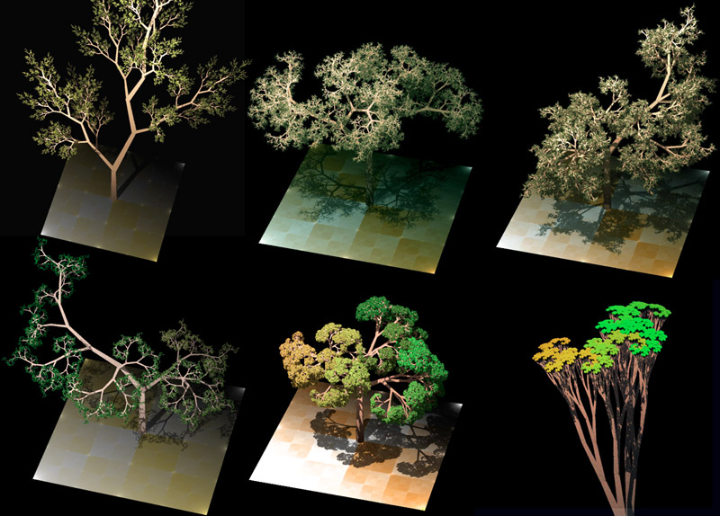
Trees are generated by the same algorithm with random tweaks to make it look diverse and realistic
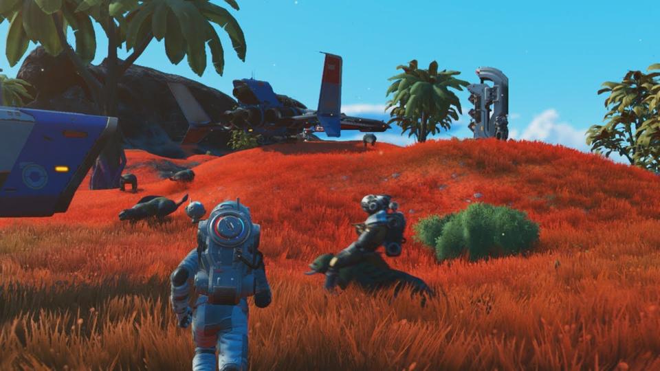
No man’s sky uses procedural generation to create the terrain, flora and fauna
This video below explains in details how you procedurally generate terrain
Personalities
Procedurally-generated content can add detail and depth to characters and story line . The personality manifests as various traits, which under the surface are simple numbers that alter the balance in a character’s decision. But because the systems revolve around relationships and behavior, these traits combine in fascinating, dramatic storyline at the center of medieval power dynamics in Crusader King II.
Another example is Sim. In Sim, you can create the characters each with its own set of traits. You can direct your Sim to do certain task but when letting on auto mode, your Sim will act its own with the inclination which suits its personality.
Game mechanics
Splunkey is a familiar but not so typical platform arcade game. Instead of forming a fixed set of levels, splunkey has a fixed set of rules for its mechanics and underlying system. The player will not be able to predict which challenge come next.
The level is almost unique with a pseudo random placement of enemies, shopkeepers, items, cave walls, and other elements. This gives the player an element of surprises and outcomes.
Exploration and Interation
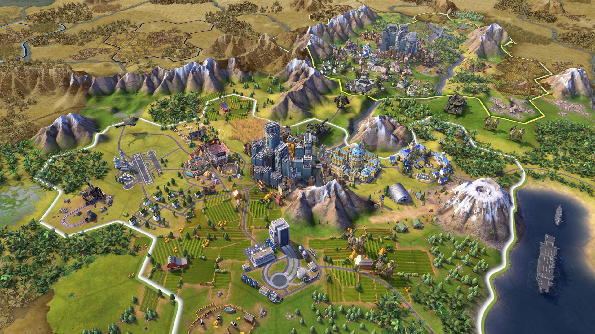
The Cilivilization series is like a big board chess game, except the maps and the game conditions are totally different from one game to another. Each player is handed a different map at the start. Playing the game is like answering a series of questions where each question is totally different every time you are asked. The choice eventually lead to an unique and totally different series of interesting situation choices each time. You will never know which civilizations you will face at the start or which challenge are you going to fight against. The possibilities are endless.
AI
In this era of escalated innovation in AI, researchers has designed an AI called Angelina. Angelina can create game by herself using procedural generation. Angelina can generate various arcade games with textures and self created mechanics.
She has also participated in game jams and create different games based on a theme word or phrase.
You can explore games created by Angelina in the link below
https://gamesbyangelina.itch.io/
Source: Gamasutra, Wikipedia, NewsAtlas
From each element stiffness matrix, we can construct the global K stiffness matrix
def ConstructGlobalK(nodes, elements):
    rowCt = 2 * len(nodes)
    colCt = 2 * len(nodes)
    globalK = np.zeros((rowCt,colCt))
    for element in elements:
        k = element.GetElementStiffness()
        triplets = element.GetTriplets(k)
        for triplet in triplets:
            tripC = rs.PointCoordinates(triplet)
            globalK[tripC[0]][tripC[1]] = tripC[2]
    return globalK
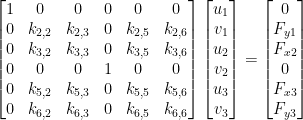
However, we are not complete yet. We need to apply constraints so we can solve the displacement vector. Displacement of constrained nodes are always zero. Consider this equation, on the left hand we have a global stiffness matrix and displacement vector, the right side is the force vector.
To constrain the node, the corresponding element of the matrix should be set to 1, and all elements in that row and column should be set to zero. There should not be any external forces acting on the constrained node in constrained direction.
Below is the code for applying constraints
def ApplyConstraint(globalK):
    conIndices = GetConstraintIndices()
    rowSize = np.size(globalK, 0)
    colSize = np.size(globalK, 1)
    for i in range(rowSize):
        for j in range(colSize):
            for index in conIndices:
                if (i == index or j == index):
                    globalK[i][j] = 1.0 if i == j else 0.0
    return globalK
Recall


We already have stiffness matrix and vector of loads. Now we can find the vector of displacements by solving the equation above
displacements = np.linalg.solve(globalK, loads)
Now we have solved the equations, we might want to visualize the result, finding the displacement vector in each node.
def GetNodeDisplacements(nodes, displacements):
    nodeDisps = []
    for i in range(0,len(nodes)):
        #this is actually add vector but add vector is not available in Rhino5 32bit
        v = rs.AddPoint( displacements[2 * i + 0], displacements[2 * i + 1], 0)
        nodeDisps.append(v)
    return nodeDisps
There we have a list of displacement vectors correspond with each node. We can also calculate the stress
stresses = []
for element in elements:
    nodeIds = element.NodeIds
    delta = np.zeros(6)
    delta[0] = displacements[2 * nodeIds[0]]
    delta[1] = displacements[2 * nodeIds[0] + 1]
    delta[2] = displacements[2 * nodeIds[1]]
    delta[3] = displacements[2 * nodeIds[1] + 1]
    delta[4] = displacements[2 * nodeIds[2]]
    delta[5] = displacements[2 * nodeIds[2] + 1]
    sigma1 = np.dot(elasM, element.GetMatrixB(element.GetMatrixC()))
    sigma = np.dot(sigma1, delta)
    sigmaCal = sigma[0] * sigma[0] - sigma[0] * sigma[1] + sigma[1] * sigma[1] + 3 * sigma[2] * sigma[2]
    sigma_mises = math.sqrt(sigmaCal)
    stresses.append(sigma_mises)
With a list of displacement vectors and list of stress value, we can visualize the result in Rhino using grasshopper display tools

Stress Display

Displacement Display

As explained in the previous post, to calculate element stiffness, we need to find the 3 matrix: D, C and B
Let’s find D first
def GetElascityMatrixD(matInfo):
   poisson = matInfo[0]
   youngModul = matInfo[1]
   matrix = np.zeros((3,3))
   matrix[0][0] = 1
   matrix[0][1] = poisson
   matrix[1][0] = poisson
   matrix[1][1] = 1
   matrix[2][2] = (1 - poisson)/2
   mult = youngModul/(1 - math.pow(poisson,2))
   elasM = mult * matrix
   return elasM
Matrix B and C are element so I wrote the methods to calculate B and C in class Element
Recall
and B i the second matrix in this
where
and element stiffness is
The methods of finding C, B and K are below. All of them are in element class
class Element:
    def __init__(self, elemNodes, nodeIds):
        self.Nodes = elemNodes
        self.NodeIds = nodeIds
    def GetMatrixC(self):
        col1 = []
        colx = []
        coly = []
        for i in range(len(self.Nodes)):
                col1.append(1)
                colx.append(self.Nodes[i].X)
                coly.append(self.Nodes[i].Y)
        matrixC = [col1, colx, coly]
        return matrixC
    def GetMatrixB(self, matrixC):
        C = matrixC
        IC = np.linalg.inv(C)
        B = np.zeros((3,6))
        for i in range(3):
            B[0][2 * i + 0] = IC[1][ i]
            B[0][2 * i + 1] = 0.0
            B[1][ 2 * i + 0] = 0
            B[1][2 * i + 1] = IC[2][i]
            B[2][2 * i + 0] = IC[2][i]
            B[2][2 * i + 1] = IC[1][i]
        return B
    def GetElementStiffness(self):
        C = self.GetMatrixC()
        B = self.GetMatrixB(C)
        D = GetElascityMatrixD(matInfo)
        BT = np.matrix.transpose(B)
        CDet = np.linalg.det(C)
        mult1 = np.dot( BT , D)
        mult2 = np.dot(mult1, B)
        K = mult2 * CDet * 1/2
        return K
We are going to use element stiffness to calculate global stiffness. For the ease of usage later on, we store element stiffness matrix together with its corresponding indices in the global stiffness matrix in a triplet. That means, for each element, we will have 3 triplets, each correspond to a vertex of that triangulated matrix. In that triplet, the first two items are nodeId positions, the last is its corresponding value in element stiffness. In this case, I use point3d as triple, it is not a point but simply a way to store 3 number all at once. Note that this GetTriplets method also nested inside Element Class
    #Calculate Stiffness Matrix
    def GetTriplets(self, K):
        triplets = []
        for i in range(0, 3):
            for j in range(0,3):
                t11 = rs.AddPoint( 2 * self.NodeIds[i] + 0, 2* self.NodeIds[j] + 0, K[2 * i + 0][2 * j + 0])
                t12 = rs.AddPoint( 2 * self.NodeIds[i] + 0, 2* self.NodeIds[j] + 1, K[2 * i + 0][2 * j + 1])
                t21 = rs.AddPoint( 2 * self.NodeIds[i] + 1, 2 * self.NodeIds[j] + 0, K[2 * i + 1][2 * j + 0])
                t22 = rs.AddPoint( 2* self.NodeIds[i] + 1, 2* self.NodeIds[j] + 1, K[2 * i + 1][2 * j + 1])
                triplets.append(t11)
                triplets.append(t12)
                triplets.append(t21)
                triplets.append(t22)
        return triplets
Now we have all the element stiffness information, we are ready to put them together to calculate the global stiffness and deformation
And….here we go, to the most complicated part of the code, calculation!
The ultimate goal of the structural FEA is to find out the deflection, and in computer terms, that would be the displacement of each node.
Link: https://podgorskiy.com/spblog/304/writing-a-fem-solver-in-less-the-180-lines-of-code
Since strain is a linear function of stress, displacement of each node is a linear function of applied forces. That is expressed by the equations below:
The global stiff matrix is calculated from each element stiff matrix. In order to find the nodal displacement, we start with an equation of the work done by nodal forces:
After some mathematical manipulations, we have:
k is element matrix. D is elasticity matrix. B and C will be explained further.
where v is poisson ratio.
Shape functions
If displacements of nodes are given, then displacement in any point of element can be obtained by the following equation
where [N] is a matrix of functions of position (x, y). u and v are components of the displacement that can be interpolated dependently. For simplicity, I take u and v as the global x vector and y vector, which i guess that’s why i have to put my geometry at the origin in order for the algorithm to work
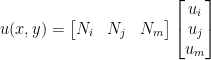
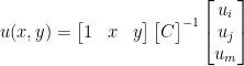
For three-node linear element, interpolation is linear. To interpolate function, we need to find an equation of the following form: (Note: think of i, j and m as each node of the triangle elememt)
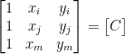
We denote C as
we therefore have:
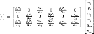
B is defined as the matrix in this equation:
Apply partial differentiation to the above equation we have
Rearrange the equation above, we can deduce:
By finding C, we can find B.
Now we have known the equations for B and C. Let’s find them in the code in the next post!
I finally got to write my own FEA code. Always wanted to do so but dreadful because I’m easily distracted and need a good time to focus on this.
Without a background in engineering yet working in an engineering company, I hope writing FEA can help me understand the engineering math.
I mainly follow this article right here and translate it to python. I will eventually upload my code to git but for now I will copy paste the pieces of my code here.
https://podgorskiy.com/spblog/304/writing-a-fem-solver-in-less-the-180-lines-of-code
I use the platform I’m most familiar with, Rhino Grasshopper which have existing methods to define and use mesh. However, I have to use Rhino 5 32bit this time because I want to use numpy for matrix calculation. I have covered the installation in a post below
Inputs
To start a FEA we need boundaries conditions:
A good triangulated mesh
Nodes which are mesh vertices
Support Conditions (nodes that are restrained)
Loading Conditions (loading vectors, loadPts)
Material Info (Poisson Ratio and Young Modulus)
Below is my set up in grasshopper

I position the mesh at origin

Set Up
In order to calculate efficiently, we need to do some “prepping”. We will set up list of nodes, edges, list of loads, list of constraints and list of elements (an element is a triangulated face)
Nodes: The input nodes currently are point3d. However, for convenience, we often refer to the nodes using its index. Whenever the situation arise, I use index to call out the nodes.
Edges: I store the indexes of the line’s start point and end point in a value pair
def GetEdges(mesh):
   edges = [] #list of vertex indices that make up the edges

   for i in range(mesh.TopologyEdges.Count):
       vPair = mesh.TopologyEdges.GetTopologyVertices(i)
       vPairPython = (vPair.I, vPair.J)
       edges.append(vPairPython)
   return edges
Loads: For loads, I need to store them in an array twice the size of the nodes array. Alternate items of the array are X and Y coordinates of the load vector
def GetLoads(nodes, loadPts, loadVs):
     loads = [0] * (len(nodes) * 2)
     for i in range(len(nodes)):
        for j in range(len(loadPts)):
          loadV = loadVs[j]
          dist = rs.Distance(loadPts[j],nodes[i])
          if dist < 0.001:
             loads[2 * i + 0] = loadV.X
             loads[2 * i + 1] = loadV.Y
      return loads
Constraints: I define a class for constraint where type is indicated by integer (1 is for constraint, x, 2 is for y, 3 is for both), node is point3d.
class Constraint:
    def __init__(self, type, node):
        self.Type = type
        self.Node = node
def GetConstraints(supportBoundaries, supportConds, nodes):
    constraints = []

    for i in range(len(nodes)):
        for j in range(len(supportBoundaries)):
           if rs.PointInPlanarClosedCurve(nodes[i], supportBoundaries[j]) == 1:
                con = Constraint(supportConds[j], i)
                constraints.append(con)
    return constraints
Elements: I created Element object woth properties are Nodes and NodeIds
class Element:
      def __init__(self, elemNodes, nodeIds):
           self.Nodes = elemNodes
           self.NodeIds = nodeIds
def GetElements(mesh):
      faceCt = rs.MeshFaceCount(mesh)
      elements = []
      for i in range(faceCt):
         faceVerticeIDs = rs.MeshFaceVertices(mesh)[i]
         nodeIds = faceVerticeIDs[:-1]
         elemNodes = [nodes[nodeIds[0]], nodes[nodeIds[1]], nodes[nodeIds[2]]]
         element = Element(elemNodes, nodeIds)
         elements.append(element)
      return elements
To list out all of them we have:
edges = GetEdges(mesh)
loads = GetLoads(nodes, loadPts, loadVs)
constraints = GetConstraints(supportBoundaries,supportConds, nodes ) #(restraintType, id)
elements = GetElements(mesh)
And…you’re done setting up the items to start on doing some math. I will cover the calculation/matrix manipulations in the next post
As things get crazy because of the virus right now, the world wide lockdown seem to boost some views for this blog which has always been hidden in this very small corner of the internet. And as i am almost 100% locked in the house now, I should dedicate a bit more time to this blog. I decided not only focus on the tech side but also more on the theory, information bits, partly because some tech requires me much more time and dedication to discover and master before I can write a proper post.
The topic today is about high tech in fashion. Although I am not so much a well dressed and highly fashionable girl, fashion design is nevertheless fascinating. Fashion is fast, quick and more approachable, more appealing to the mass. Due to its fast nature, (I find) fashion is more updated to the current culture. Unlike art, fashion design has to uphold certain basic function, which make it more relevant to architecture and interesting to study. I will start this series with MetGala 2016 as an introduction then introduce some high tech fashion designers subsequently
ManusxMachina Met Gala
The Met Gala, formally called the Costume Institute Gala and also known as the Met Ball, is an annual fundraising gala in the benefit of the Metropolitan Museum of Art’s Costume Institute in New York City. (Source: Wikipedia). Every year, an exhibition is held and a gala filled with celebrities is organized. In 2016, the Met Gala theme was ManusxMachina.

In the words of the curator, ManusxMachina explores how fashion designers are reconciling the handmade and the machine-made in the creation of haute couture and avant-garde ready-to-wear. ManusxMachina is not necessarily about “robotic clothing”, but rather about subtle hidden technologies:
“Traditionally, the handmade has been seen as being about luxury whereas the machine has been about progress and the future. On the other side, it’s been about mediocrity and dehumanization. Those values sometimes dont really hold up”
Hmm the statement draws some parallel to the architecture world. Since the industrial revolution, buildings starts being made by machine, with parts made from mass production. The machine-made standardised building quickly fill up and rapidly form the cities today. Are they seen as mediocrity and dehumanization too? Or are they seen as futuristic. Again, these values do not have to hold up. Technology should open us to more possibility and diversity in design, rather than sticking them to certain connotation.
For more details, check out the link below!
https://www.metmuseum.org/exhibitions/listings/2016/manus-x-machina
Issey Miyake
Issey Miyake is a Japanese designer. Besides designing sculptural clothing that make you look like an origami penguine, Issey Miyake has many recognisable works such as the triangulated folding bag and Steve Job’s turtleneck


Miyake’s design process explores the fundamental relationship between the body, the cloth that covers it, and the space and room that is created between these elements, divesting itself of the labels of “East” or “West”. He is interested in making innovative improvements to the traditional techniques, breathing new life to historic techniques to respond to the demand of times.
Issey Miyake most notable works are:
Pleating: A technique that allows both flexibility of movement for the wearer as well as ease of care and production using light weight material.
APOC (A piece of cloth): A-POC create fabric and clothing from a single thread with a high degree of variation using computerized instructions.
Source: http://mds.isseymiyake.com/im/en/work/
Iris Van Herpen
Of course we cannot forget to mention Iris Van Herpen when it comes to high tech fashion. Iris Van Herpen is a Dutch fashion designer who is the pioneer in utilizing 3D printing as a garment construction technique. Her multi disciplinary technique has led to collaboration with various designers such as Jolan vander Weil, Neri Oxman and architects such as Philip Beesley and Benthem and Crowel Architects.
What I’m most impressed is not the technology she used but her design process where she incorporate the technology in the design process. The inspiration come directly from the designer’s interest and spring into idea through conceptualizing her own personal sensory, perception of the world. Using technology, Iris is able express and let that idea evolve into physical object by itself.
“When I work on my design, it’s about finding a moment for a woman rather than finding an identity” “A lot of collections start from experiment and a lot of things start from a failure as well”
The results are absolutely stunning. “The designs are so ethereal yet futuristic, fragile yet fierce, delicate yet powerful.” (from an internet comment)
Ying Gao
Ying Gao is a Chinese Montreal based fashion designer. She has many exhinition around the world and featured in prestigious international media.
“Ying Gao questions our assumptions about clothing by combining fashion design, product design and media design. She explores the construction of the garment, taking her inspiration from the transformations of the social and urban environment. Design is the medium, situated in the technological and the textile realm : sensory technologies allow garments to become more poetic and interactive.”
Source: yingao.ca
Other designers you can search for include Junya Watanabe, Jean-Paul Gaultier, or Anouk Wipprecht
Hi all,
After a painful process of installling numpy. I would summarize my process as below. Hope it is helpful to everyone.
http://code.enthought.com/.iron/eggs/index.html
Download all of them to your Downloads folder
“C:\Program Files (x86)\IronPython 2.7\ipy.exe” IronPython_numpy_scipy.py --install
It will return an “egginst” error. That’s because you do not have that module yet.
Copy the egginst folder to downloads
Although I really enjoy learning, certain topic could be a long and arduous journey which often land me scrolling through the internet looking at dogs and cats or random youtube music videos. Thus, instead of researching or learning a computational topic in depth today, the designer in me decided to write some cheap quick and easy code but able to get something appear on my screen just for the cheap thrill of feeling like a “CoMpUtAtIoNaL DeSiGnEr”.
Beside being a computational designer, I am also a recent practitioner of yoga. While trying out new and more challenging poses, I often find the process of balancing as something iterative. Once finding the balance, the right spot, the pose become much easier and require much less strength. Inspired by the practice, I been trying to bring images of yoga poses photo to a 3D vector skeleton in Rhino.
I run the yoga pose image through two algorithm: poseNet and denseDepth. poseNet returns the human skeleton, with the “coordinates” of the joints. These coordinates are then mapped onto denseDepth image, return us the “brightness” of that pixels. All these numbers are then brought into Rhino and make up a 3D human skeleton.

Original Image

PoseNet

Dense Depth

Dense Depth with mapped joints (zoom in closely)


3D result…sorry for the exploded head hehe.
I understand that there are much better algorithm to do this such as densepose and the result looks very different from the image, but hey this is just an attempt for me to have some fun!

![\left [ K \right ] \left [ \delta \right ] = \left [ R \right ]](https://s0.wp.com/latex.php?latex=%20%5Cleft%20%5B%20K%20%5Cright%20%5D%20%5Cleft%20%5B%20%5Cdelta%20%5Cright%20%5D%20%20%3D%20%20%5Cleft%20%5B%20R%20%5Cright%20%5D&bg=ffffff&fg=000000&s=0 "\left [ K \right ] \left [ \delta \right ] = \left [ R \right ]")
![\left [ D \right ] = \cfrac{E}{1-\nu^2} \begin{bmatrix} 1 & \nu & 0 \\ \nu & 1 & 0 \\ 0 & 0 & \cfrac{1-\nu}{2} \end{bmatrix}](https://s0.wp.com/latex.php?latex=%20%5Cleft%20%5B%20D%20%5Cright%20%5D%20%3D%20%20%5Ccfrac%7BE%7D%7B1-%5Cnu%5E2%7D%20%20%20%5Cbegin%7Bbmatrix%7D%20%20%20%201%20%26%20%5Cnu%20%26%200%20%5C%5C%20%20%20%5Cnu%20%26%201%20%26%200%20%5C%5C%20%20%20%200%20%26%200%20%26%20%5Ccfrac%7B1-%5Cnu%7D%7B2%7D%20%20%20%5Cend%7Bbmatrix%7D%20&bg=ffffff&fg=000000&s=0 "\left [ D \right ] = \cfrac{E}{1-\nu^2} \begin{bmatrix} 1 & \nu & 0 \\ \nu & 1 & 0 \\ 0 & 0 & \cfrac{1-\nu}{2} \end{bmatrix}")


![\begin{bmatrix} u(x,y) \\ v(x,y) \end{bmatrix} = \left [ N \right ] \left [\delta \right ]^e](https://s0.wp.com/latex.php?latex=%20%20%5Cbegin%7Bbmatrix%7D%20u%28x%2Cy%29%20%5C%5C%20v%28x%2Cy%29%20%5Cend%7Bbmatrix%7D%20%20%20%3D%20%5Cleft%20%5B%20N%20%5Cright%20%5D%20%5Cleft%20%5B%5Cdelta%20%5Cright%20%5D%5Ee%20&bg=ffffff&fg=000000&s=0 "\begin{bmatrix} u(x,y) \\ v(x,y) \end{bmatrix} = \left [ N \right ] \left [\delta \right ]^e")